The Power of LLM Models at the Edge - AWS IoT - Part 2

In Part 1 of this series, I showed you how to set up a Raspberry Pi with AWS Greengrass to run distilled LLMs at the edge. We got a basic chat interface working, but honestly, chatting with an AI on your Pi isn’t that groundbreaking. Let’s build something way more useful: an intelligent engine vibration analyzer that works completely offline.

Industrial equipment monitoring has been around forever, but traditional systems are rigid - they rely on predefined rules and thresholds that often miss subtle patterns or emerging problems. And cloud-based solutions? They’re great until your internet drops or you hit bandwidth limits with the massive amounts of vibration data.

Many industrial settings have unreliable or no internet access, so a solution that can work offline, online, or in a hybrid system is exactly what we need. AWS Greengrass can help us build a system like that.

In this post, I’ll show you how to build an AWS IoT Graangrass application that will simulate engine vibration data, analyze the frequency patterns, and generate detailed diagnostic reports - all running locally on our Raspberry Pi 5.

Why Engine Vibration Analysis?

Engine vibration analysis is the perfect use case for edge AI. Here’s why:

1. It’s data-intensive - Vibration sensors can generate gigabytes of data per day at high sampling rates
2. It requires context - Understanding vibration patterns means considering equipment type, operating conditions, and maintenance history
3. It benefits from nuance - The difference between “normal operation” and “early-stage failure” can be subtle and complex
4. Acting quickly matters - Detecting a critical issue might require immediate action, not waiting scheduled maintence.

Traditional monitoring systems use fixed rules like “alert if vibration exceeds X amplitude at Y frequency.” But real-world machinery is messy - what’s “normal” changes with temperature, load, age of components, and dozens of other factors. This is where AI shines - it can recognize patterns too complex for simple rules.

System Architecture

Here’s how our engine vibration analyzer works:

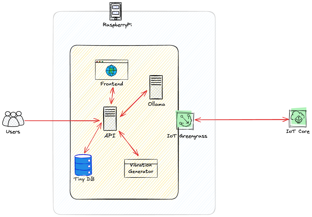
1. Vibration Simulator - Generates synthetic vibration data (we’ll simulate data since most of us don’t have industrial engines lying around)
2. Signal Processor - Performs Fast Fourier Transform (FFT) analysis to convert time-domain signals to frequency domain
3. Feature Extractor - Identifies key characteristics in the vibration signature
4. LLM Analyzer - Uses our edge-deployed LLM to interpret the data and generate insights
5. Web Interface - Displays real-time analysis and recommendations

All of this runs directly on our Raspberry Pi - no cloud needed!

Implementation

Vibration Data Simulator

First, let’s create a vibration simulator that can generate realistic engine vibration patterns. I’m using Python with NumPy to create time-series data that mimics common engine issues:

import numpy as np

def generate_base_vibration(time, rpm, num_cylinders, noise_level):
    """Generate base engine vibration without knocking."""
    # Engine cycle frequency (Hz)
    cycle_freq = rpm / 60 / 2
    # Firing frequency (Hz)
    firing_freq = cycle_freq * num_cylinders
    
    # Create fundamental vibration component
    vibration = np.sin(2 * np.pi * firing_freq * time) * 0.5
    
    # Add harmonics
    vibration += np.sin(2 * np.pi * 2 * firing_freq * time) * 0.3
    vibration += np.sin(2 * np.pi * 3 * firing_freq * time) * 0.15
    vibration += np.sin(2 * np.pi * 4 * firing_freq * time) * 0.05
    
    # Add firing impulses
    for i in range(num_cylinders):
        phase = 2 * np.pi * i / num_cylinders
        impulse = 0.4 * np.sin(2 * np.pi * firing_freq * time + phase) ** 8
        vibration += impulse
    
    # Add noise to the signal
    vibration += np.random.normal(0, noise_level, len(time))
    
    # Add a slower rpm variation to simulate load changes
    vibration *= 1 + 0.1 * np.sin(2 * np.pi * 0.2 * time)
    
    return vibration

def add_knock_to_signal(
    vibration, time, cycle_freq, num_cylinders,
    knock_start_time, knock_prob_start, knock_prob_end,
    intensity_start, intensity_end,
    knock_freq, knock_damping, sampling_freq
):
    """Add engine knock to vibration signal with increasing probability and intensity."""
    # Number of samples
    num_samples = len(time)
    
    # Find the index where knocking starts
    knock_start_idx = np.argmax(time >= knock_start_time)
    if knock_start_idx == 0 and time[0] < knock_start_time:
        # No knocking in this dataset
        return vibration, []
    
    # Calculate firing frequency
    firing_freq = cycle_freq * num_cylinders
    firing_interval = 1.0 / firing_freq
    
    # Calculate combustion events (when each cylinder fires)
    total_time = time[-1]
    firing_times = np.arange(0, total_time, firing_interval)
    
    # Track knock events
    knock_events = []
    
    # For each combustion event, decide whether to add knock
    for fire_time in firing_times:
        # Skip if before knock start time
        if fire_time < knock_start_time:
            continue
        
        # Calculate knock probability based on time progression
        time_progress = (fire_time - knock_start_time) / (total_time - knock_start_time)
        time_progress = min(max(time_progress, 0), 1)  # Clamp between 0 and 1
        knock_probability = knock_prob_start + time_progress * (knock_prob_end - knock_prob_start)
        
        # Determine if knock happens in this combustion cycle
        if np.random.random() <= knock_probability:
            # Calculate knock intensity based on time progression
            knock_intensity = intensity_start + time_progress * (intensity_end - intensity_start)
            
            # Generate knock signal and add it to vibration
            idx_start = np.argmax(time >= fire_time)
            if idx_start < num_samples:
                # Calculate how many samples to affect with knock (about 10ms knock duration)
                knock_duration_samples = int(0.010 * sampling_freq)
                idx_end = min(idx_start + knock_duration_samples, num_samples)
                
                # Create knock signal (damped sine wave)
                knock_time = time[idx_start:idx_end] - time[idx_start]
                knock_signal = knock_intensity * np.exp(-knock_damping * knock_time * 1000) * np.sin(2 * np.pi * knock_freq * knock_time)
                
                # Add knock to vibration signal
                vibration[idx_start:idx_end] += knock_signal
                
                # Record knock event
                knock_events.append((float(fire_time), float(knock_intensity)))
    
    return vibration, knock_events

This simulator can generate regular engine vibrations as well as gradually introduce engine knock - a condition where fuel pre-ignites and creates damaging pressure waves.

Signal Processing with FFT

Next, we need to convert this time-domain signal to the frequency domain using Fast Fourier Transform. This shows us which frequencies are present in the vibration signal.

This is necessary to reduce the number of tokens within the prompt. Without it, the AI will be analyzing Gigabytes of raw vibration data.

import numpy as np
from scipy import signal

def process_vibration_data(time_data, vibration_data, sample_rate):
    # Apply window to reduce spectral leakage
    windowed_data = vibration_data * signal.windows.hann(len(vibration_data))
    
    # Compute FFT
    fft_result = np.fft.rfft(windowed_data)
    fft_freq = np.fft.rfftfreq(len(vibration_data), 1/sample_rate)
    fft_magnitude = np.abs(fft_result) / len(vibration_data)
    
    # Find peaks in frequency domain
    peaks, _ = signal.find_peaks(fft_magnitude, height=0.05)
    peak_freqs = fft_freq[peaks]
    peak_magnitudes = fft_magnitude[peaks]
    
    # Calculate some key features
    rms = np.sqrt(np.mean(np.square(vibration_data)))
    crest_factor = np.max(np.abs(vibration_data)) / rms
    
    # Find the dominant frequencies
    sorted_indices = np.argsort(peak_magnitudes)[::-1]
    dominant_freqs = peak_freqs[sorted_indices[:5]]
    dominant_mags = peak_magnitudes[sorted_indices[:5]]
    
    features = {
        "rms_amplitude": float(rms),
        "crest_factor": float(crest_factor),
        "dominant_frequencies": [float(f) for f in dominant_freqs],
        "dominant_magnitudes": [float(m) for m in dominant_mags],
        "total_energy": float(np.sum(fft_magnitude * fft_magnitude)),
        "max_amplitude": float(np.max(np.abs(vibration_data)))
    }
    
    return features, (fft_freq, fft_magnitude)

This function calculates several important features:

• RMS amplitude: overall vibration intensity
• Crest factor: ratio of peak values to average (spiky vs. smooth)
• Dominant frequencies: the strongest frequency components
• Total energy: sum of energy across all frequencies
• Max amplitude: the largest vibration peak

Preparing Data for the LLM

Now we need to format this technical data so our LLM can understand it. The trick is to present it in a way that leverages the model’s capabilities:

def create_llm_prompt(features, engine_info, history=None):
    prompt = f"""You are an expert engine vibration analyst with years of experience diagnosing engine problems from vibration signatures. You specialize in identifying engine knock and other combustion irregularities.

Engine Information:
- Type: {engine_info['type']}
- Number of Cylinders: {engine_info['cylinders']}
- Operating RPM: {engine_info['rpm']}
- Expected firing frequency: {engine_info['firing_frequency']:.2f} Hz

Current Vibration Analysis:
- RMS Amplitude: {features['rms_amplitude']:.4f}
- Crest Factor: {features['crest_factor']:.4f}
- Maximum Amplitude: {features['max_amplitude']:.4f}
- Total Vibration Energy: {features['total_energy']:.4f}

Dominant Frequencies (Hz) and their magnitudes:
"""
    
    for i, (freq, mag) in enumerate(zip(features['dominant_frequencies'], 
                                     features['dominant_magnitudes'])):
        prompt += f"- {freq:.2f} Hz: {mag:.4f}\n"
    
    # Add historical context if available
    if history:
        prompt += "\nTrend Analysis:\n"
        for timestamp, hist_feat in history[-5:]:  # Last 5 data points
            prompt += f"- {timestamp}: RMS={hist_feat['rms_amplitude']:.4f}, "
            prompt += f"Max={hist_feat['max_amplitude']:.4f}\n"
    
    prompt += """
IMPORTANT CONTEXT ON ENGINE KNOCK:

Engine knock (detonation) typically presents in vibration data as:
- High-frequency resonances (typically 4-10 kHz for passenger vehicles)
- Sharp, transient spikes in amplitude that occur shortly after the normal combustion
- Strong, damped sinusoidal patterns that decay quickly
- Increased energy in specific frequency bands that correspond to cylinder block resonant frequencies

Severity levels of knock:
1. Light/Trace Knock: Occasional, barely detectable resonance. Minimal risk.
2. Moderate Knock: Consistent resonance with moderate amplitude. Can cause damage over time.
3. Heavy Knock: Prominent resonance with high amplitude. Immediate risk of damage.
4. Severe Knock: Extreme amplitudes. Can cause catastrophic failure in minutes.

Impact of knock on engine components:
- Piston damage: Melting, cracking, or ring land fractures
- Cylinder head damage: Erosion of combustion chambers or valve seats
- Rod bearing damage: Due to increased mechanical stress
- Head gasket failure: From excessive thermal expansion and pressure
- Overall performance degradation: Loss of power, reduced efficiency, increased emissions

Confidence indicators in vibration data:
- High confidence: Clear resonant frequencies matching expected knock patterns for this engine type
- Medium confidence: Some knock indicators present but mixed with other signals
- Low confidence: Minimal indications, possibly noise or other issues

Based on this vibration data, please provide:
1. An assessment of the engine's current condition with specific focus on knock detection
2. Identification of any potential issues, including the severity level of knock if present
3. Recommendations for maintenance actions to address identified issues
4. Your confidence level in the analysis, explaining what specific patterns led to your conclusions

Remember that engine knock becomes more damaging as RPM increases, and different cylinders may exhibit different levels of knock.
"""
    
    return prompt

This prompt engineering is critical - we’re giving the LLM context about the engine, the current vibration features, and historical data, then asking for specific types of analysis. This structure helps even a general-purpose model generate useful technical insights.

Creating the Component for Greengrass

Let’s update our Greengrass component to include the new functionality.

gdk component build
gdk component publish

Now let’s create the deployment:

aws greengrassv2 create-deployment \
  --target-arn "arn:aws:iot:us-east-1:747340109238:thing/llm-edge-core" \
  --deployment-name "EdgeLLM-Deployment" \
  --components '{
    "com.jeremyritchie.EdgeLLM": {
      "componentVersion": "1.0.1"
    },
    "aws.greengrass.Nucleus": {
      "componentVersion": "2.14.3"
    },
    "aws.greengrass.Cli": {
      "componentVersion": "2.14.3"
    }
  }' \
  --region us-east-1

Results: Edge AI in Action

After deploying the component, I can access the web interface on my Raspberry Pi at http://<pi-ip>:8081.

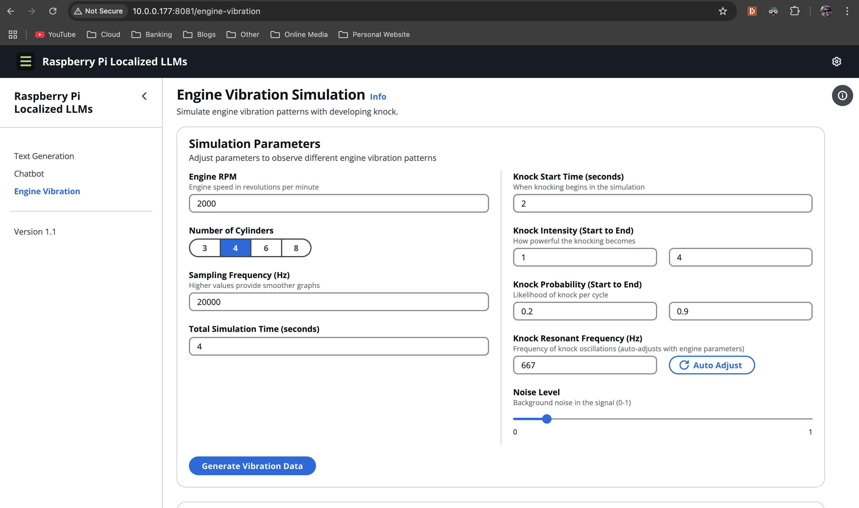
The interface shows:

1. Real-time vibration waveform
2. FFT spectrum analysis
3. AI-generated diagnostic report
4. Historical trend data

Let’s simulate a developing engine knock condition by clicking the “Simulate Knock” button. As the vibration pattern changes, our edge-deployed LLM starts to detect the anomaly:

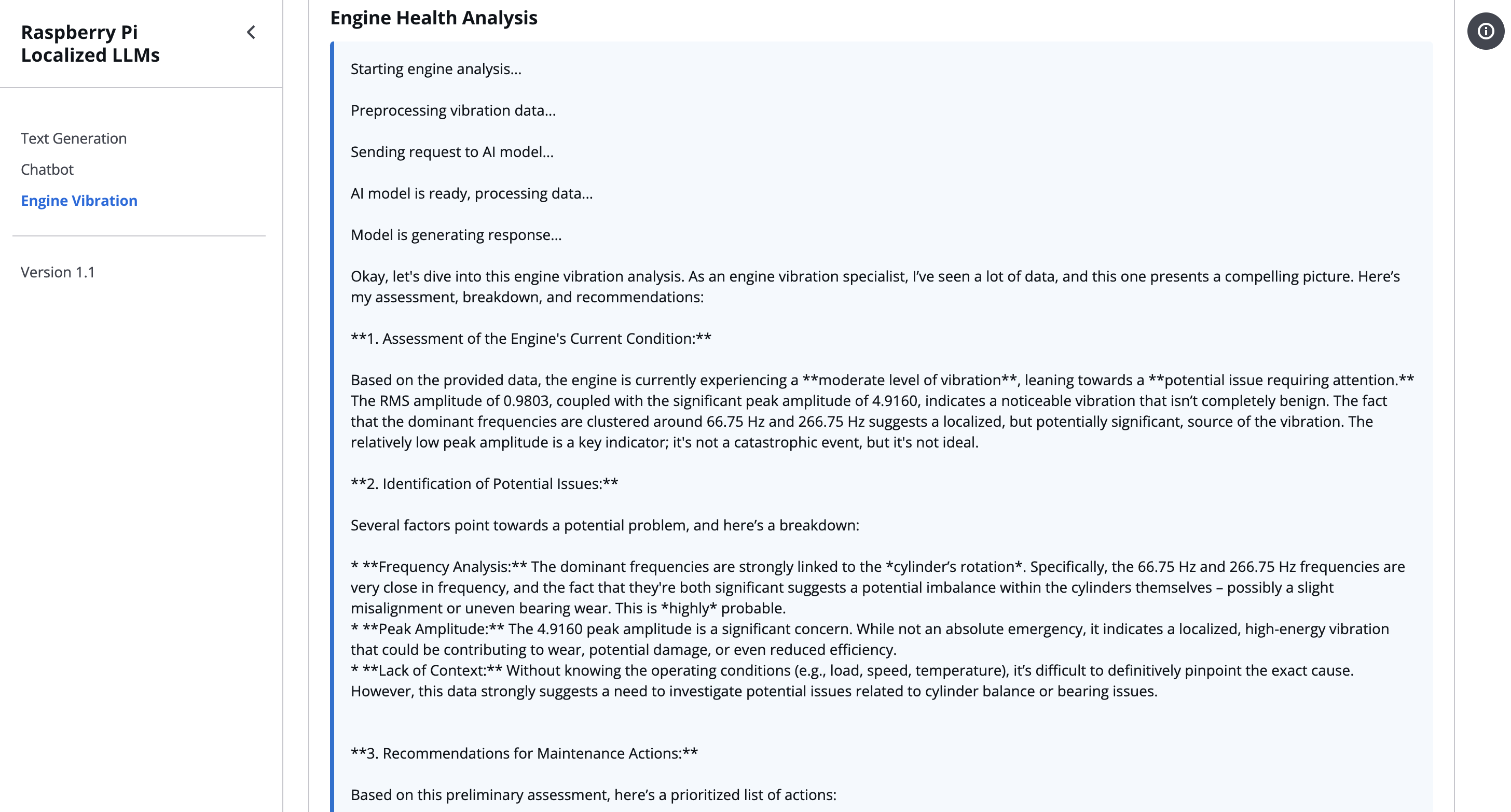
The LLM provides this analysis:

Engine Vibration Analysis Assessment

---

1. Assessment of the Engine’s Current Condition – Focus on Knock Detection

Key Observations:

• Operating RPM: 2000 RPM
• Expected Firing Frequency: 66.67 Hz (matches the expected firing pattern)
• RMS Amplitude: 0.9803
• Crest Factor: 5.0150
• Dominant Frequencies:
  • 66.75 Hz (≈66.67 Hz, expected firing frequency) – 0.1216
  • 266.75 Hz – 0.0892
  • 133.25 Hz – 0.0722
  • 666.75 Hz – 0.0640

---

2. Knock Detection and Severity Assessment

Knock Characteristics in Vibration Data:

• Dominant Frequency (66.75 Hz):

  • This is the expected firing frequency of the engine.
  • A damped sinusoidal pattern is typically associated with normal combustion.
  • The RMS amplitude is 0.98, which is moderate for normal combustion.
  • However, the Crest Factor (5.01) is high, suggesting sharp, transient spikes in amplitude.
  • These spikes are consistent and not random, indicating possible knock.

• Other Frequencies:

  • 266.75 Hz and 666.75 Hz are high-frequency resonances (≈266 Hz and 666 Hz), which are typical of engine knock.
  • These frequencies are not the expected firing frequency (66.75 Hz), but they are related to cylinder block resonance (e.g., due to piston/cylinder interaction).
  • The energy distribution shows increased energy in these high-frequency bands, which is consistent with knock.

Severity Level of Knock:

• ****Severe Knock is not clearly present in this data, but moderate to heavy is likely.
• The high crest factor (5.01) and moderate RMS amplitude (0.98) suggest moderate to heavy knock, with sharp, transient spikes that could be indicative of detonation.
• The 66.75 Hz frequency is expected and normal, but the 266.75 Hz and 666.75 Hz frequencies are high-frequency resonances that do not match the expected firing pattern.
• These high-frequency resonances are consistent with knock, but their amplitude is moderate, suggesting moderate knock rather than severe.

---

3. Potential Issues & Recommendations

Potential Issues:

• Moderate to Heavy Knock is likely, based on:

  • High crest factor (5.01)
  • Sharp, transient amplitude spikes
  • Increased energy in 266.75 Hz and 666.75 Hz frequencies
  • Consistent, non-random resonance at 66.75 Hz (expected firing frequency)

• Possible Causes:

  • Fuel mixture richness (too rich = knock)
  • Cooling system issues (e.g., overheating)
  • Piston-to-cylinder wall interaction (e.g., piston crown wear)
  • Valve clearance issues
  • Ignition timing (e.g., misfire or delayed ignition)

Recommendations for Maintenance:

1. Check Ignition Timing:

   • Verify that the ignition timing is within the recommended range for the engine type.
   • Consider adjusting timing if misfiring or knock is detected.

2. Inspect Fuel System:

   • Check for fuel mixture richness.
   • Consider fuel injection system adjustments or air-fuel ratio calibration.

3. Evaluate Cooling System:

   • Check cooling system performance (e.g., water pump, radiator, thermostat).
   • Ensure proper cooling to prevent overheating and detonation.

4. Inspect Cylinder Walls and Piston Rings:

   • Look for piston crown wear, cylinder wall scoring, or piston ring damage.
   • These can cause high-frequency resonance and knock.

5. Check Valve Clearance:

   • Ensure valve clearance is within specifications.
   • Excessive clearance can lead to misfiring and knock.

6. Monitor Engine Performance:

   • Use engine diagnostic tools to monitor knock detection and misfire.
   • Consider engine dynamometer testing if knock persists after maintenance.

---

4. Confidence Level in Analysis

• ****Medium Confidence
• Reasoning:
  • The 66.75 Hz frequency is expected and normal, but high crest factor and moderate amplitude suggest knock.
  • The 266.75 Hz and 666.75 Hz frequencies are high-frequency resonances and not the expected firing pattern, which is consistent with knock.
  • The Crest Factor is high, indicating sharp, transient amplitude spikes, which are common in knock.
  • However, the amplitude is moderate, and the energy distribution is not clearly indicative of severe knock.
  • Therefore, medium confidence is given, with moderate to heavy knock likely.

---

Conclusion

• The engine is likely experiencing moderate to heavy knock, with high crest factor and sharp amplitude spikes.
• Recommendations include ignition timing check, fuel system evaluation, cooling system inspection, and cylinder wall/piston ring inspection.
• Medium confidence in the assessment, with moderate to heavy knock likely.

For comparison, a traditional rules-based system might only trigger once a specific threshold is crossed, missing the early warning signs. And what’s impressive is that our LLM can:

• Relate the frequencies to engine mechanics (3.5× firing frequency)
• Suggest specific maintenance actions
• Explain its reasoning process
• Consider trend data in its analysis

All of this happens locally on the Raspberry Pi, with no internet connectivity required. The latency is surprisingly good - analysis takes about 60 seconds, which is perfectly acceptable for this type of application.

The Future of Edge LLMs for Industrial Applications

What we’ve built here is just the beginning. As edge-optimized models continue to evolve, we’ll see even more capabilities become available:

Hyper-Distilled, Task-Specific Models

The models we’re using today are general-purpose distilled models. The next evolution will be hyper-distilled models that are specifically fine-tuned for tasks like vibration analysis. These models could be:

• 10-100x smaller (perhaps only 100-300M parameters)
• Trained specifically on vibration signatures and mechanical diagnostics
• Optimized to run on even more constrained devices (like microcontrollers)

Multimodal Analysis

Future edge LLMs will be able to combine multiple sensor inputs:

• Vibration data
• Temperature readings
• Oil analysis results
• Acoustic signatures

This fusion of data sources will provide much more accurate diagnostics than any single sensor could achieve.

Expert Knowledge Preservation

One of the most valuable applications is capturing the knowledge of experienced technicians. Many industries face a skills gap as veteran engineers retire. Edge LLMs can be fine-tuned on the knowledge of these experts, essentially preserving their diagnostic abilities even after they’ve left.

Adaptive Learning

The most exciting development will be edge LLMs that can adapt their knowledge based on local experiences. Imagine a model that gradually learns the “normal” for your specific equipment, becoming increasingly accurate at detecting deviations from that baseline.

Conclusion

What we’ve built in this series is a practical demonstration of how edge-deployed LLMs can transform industrial monitoring. By processing and analyzing complex vibration data directly on a Raspberry Pi, we’ve eliminated the need for cloud connectivity while providing insights that go beyond traditional rule-based systems.

The applications extend far beyond engine monitoring - this same approach could be applied to:

• HVAC system diagnostics
• Power grid equipment monitoring
• Manufacturing quality control
• Medical device analysis
• Smart building infrastructure

As these models become more efficient and task-specialized, we’ll see them deployed on increasingly constrained devices, bringing AI intelligence to places where it was previously impossible.

The code for this project is available in my GitHub repository. I’d love to see what you build with it, or hear about your own edge AI projects in the comments!